
On this page you’ll find a brief introduction to R as well as some examples of the analysis that I have run using R in the last few years.
For the Analysis below I will be using the EGloss data set. This data was collected in 2014 and compares vocabulary learning by second language learners of Chinese when reading via traditional format and a gloss (http://www.mandarintools.com/dimsum.html). Below is a list of the variables in the data set.- ID – This is the unique ID for each student in the data set
- Week – This is the week in which the student did the reading. Students read one reading per week for ten weeks. The first two weeks were used a trial run and thus were not included in this data set.
- VocabWords – Each week the length of reading varied slightly, so this variable counts the number of words in the text read to control for text lenght.
- Course – There were two courses, year one (1020) and year two (2020) Chinese.
- Pre_Sum – This is the total correct score on the pre-vocabuly test. All words have two possible points, one for pinyin and one for the English.
- Post_Sum – This is the total correct score on the post-vocabuly test. All words have two possible points, one for pinyin and one for the English.
- RawGain – This is the gain score that was calculated by subtracting the pre-test scores from the post-test scores.
- Per_Pre – Because each week had a different number of vocabulary words, this is the percentage of correct vocabulary on the pre-test.
- Per_Post –Because each week had a different number of vocabulary words, this is the percentage of correct vocabulary on the post-test.
- Per_Gain – This is the percentage of vocabulary gained after each reading each week.
For more information about this data set please see the following article: 2016 – Poole, F., & Sung, K. A preliminary study on the effects of an E-gloss tool on incidental vocabulary learning when reading Chinese as a foreign language. Journal of Chinese Language Teachers Association. 51(3), 266–285.
## # A tibble: 15 × 11
##    ID     Week Format VocabWords Course Pre_Sum Post_Sum RawGain Per_Pre
##    <chr> <dbl> <chr>       <dbl>  <dbl>   <dbl>    <dbl>   <dbl>   <dbl>
##  1 10203     3 G              44   1020    46       58.5    12.5   0.523
##  2 10203     5 G              38   1020    41.5     51.5    10     0.546
##  3 10203     7 G              38   1020    39.5     46       6.5   0.520
##  4 10203     9 G              38   1020    33       39.5     6.5   0.434
##  5 10203     4 T              37   1020    52       53       1     0.703
##  6 10203     6 T              38   1020    28       42      14     0.368
##  7 10203     8 T              38   1020    31.5     41       9.5   0.414
##  8 10203    10 T              26   1020    18       35.5    17.5   0.346
##  9 10202     4 G              37   1020    52.5     65      12.5   0.709
## 10 10202     6 G              38   1020    29       45.5    16.5   0.382
## 11 10202     8 G              38   1020    27.5     41.5    14     0.362
## 12 10202    10 G              26   1020    22       29       7     0.423
## 13 10202     3 T              44   1020    30       59.5    29.5   0.341
## 14 10202     5 T              38   1020    40       51      11     0.526
## 15 10202     7 T              38   1020    37.5     50      12.5   0.493
## # ℹ 2 more variables: Per_Post <dbl>, Per_Gain <dbl>
1 A shiny App to explore the data first
2 Download R and Rstudio
3 Create a Project
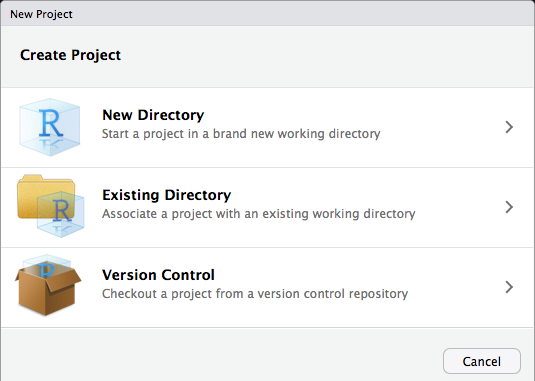
Once you have downloaded R and Rstudio. You should begin by creating a new project in RStudio. You could just simply open R studio and start coding in the console, or create a new script and start coding in the script, but creating a new Project for each data analysis project that you do will save trouble further down the road.
To start a new project open Rstudio, click File, New Project. The image below should pop up and prompt you to create a new directory or to use an existing directory. I usually just create an empty folder somewhere on my computer and then use select an existing directory.
Once you have created a new project you should see a .Rproj file in the folder that you created. In this same folder you will want to drag in whatever data file you are currently using (.csv, .spss, .xsls are all suitable among others). By creating a project and adding your data file to the folder you will a) save yourself time when importing the file into your project because you won’t have to add a long path file to your code, and b) you will make your life easier when you have to return to your analysis five months after you already completed it. More on this later.
4 Loading Data
When loading data into R you will often need to use a package for
files other than .csv. If you have not already installed a package into
your R environment, you’ll need to run the following code in the
console: install.packages("PackageName") (Don’t
forget to add the parentheses when installing a package…loading a
library does not use parentheses). After you have installed it
once, you can simply recall the package by running
library(PackageName). Below are list of the packages that
are needed for each file type.
.csv files – No Package Needed –
df <- read.table("eGloss.csv", header=TRUE, sep=",")
.xlsx files – library(readxl) –
df <- read_excel("eGlossData.xlsx") .spss
files – library(haven) –
df <- read_sav(eGlossData.spss) .sas
files – library(haven) –
df <- read_sas(eGlossData.sas)
For this project I’ll be uploading the following excel file. Remember if you create a project and add the file to the same folder as your project, you don’t need to worry about specifying the path ofthe file.
The code col_types identifies the type of variable that
each column is. So column one is a text variable, two is a numeric and
so on.
## # A tibble: 15 × 11
##    ID     Week Format VocabWords Course Pre_Sum Post_Sum RawGain Per_Pre
##    <chr> <dbl> <chr>       <dbl>  <dbl>   <dbl>    <dbl>   <dbl>   <dbl>
##  1 10203     3 G              44   1020    46       58.5    12.5   0.523
##  2 10203     5 G              38   1020    41.5     51.5    10     0.546
##  3 10203     7 G              38   1020    39.5     46       6.5   0.520
##  4 10203     9 G              38   1020    33       39.5     6.5   0.434
##  5 10203     4 T              37   1020    52       53       1     0.703
##  6 10203     6 T              38   1020    28       42      14     0.368
##  7 10203     8 T              38   1020    31.5     41       9.5   0.414
##  8 10203    10 T              26   1020    18       35.5    17.5   0.346
##  9 10202     4 G              37   1020    52.5     65      12.5   0.709
## 10 10202     6 G              38   1020    29       45.5    16.5   0.382
## 11 10202     8 G              38   1020    27.5     41.5    14     0.362
## 12 10202    10 G              26   1020    22       29       7     0.423
## 13 10202     3 T              44   1020    30       59.5    29.5   0.341
## 14 10202     5 T              38   1020    40       51      11     0.526
## 15 10202     7 T              38   1020    37.5     50      12.5   0.493
## # ℹ 2 more variables: Per_Post <dbl>, Per_Gain <dbl>
4.1 Renaming your Data
Now that I have my data uploaded, I need to rename it. Renamining
your data to something simple and generic can be very useful in R.
First, if you keep the name eGlossData, then everytime you
want to run an analysis or use a variable from this data set you’ll need
to either use attach() and detach() functions,
or you’ll need to type out the entire name. It doesn’t seem like a long
name now, but after you type it out 100 times, you’ll wish you had a
smaller name. Secondly, if you use a generic name like df
(data frame) and if you save your code into a script within your
project, then the next time you want to run your script with say another
data set, you’ll just need to rename your new data set to
df and then all of your code should run smoothly… provided
that the data is in a similar format.
Renaming data sets in R is pretty simple. See code below.
df <- glossdf.
5 Transorming Data
5.1 Creating New Variables
In the this data set we already have a variable called “RawGain.” But to practice we are going to create another variable simply called gain to show a) how to create new variables and b) how to do simple arithmetic in R.
To create a new variable simple use the $ after your
data set, and then type in a variable that is not currently in your data
set. Then use the arror <- to define what will be stored
in the variable. See examples below.
df$gain <- df$Post_Sum - df$Pre_SumTo check our answer we will look at the first 15 cases of each
variable using the head command.
head(df$RawGain, n=15)## [1] 12.5 10.0 6.5 6.5 1.0 14.0 9.5 17.5 12.5 16.5 14.0 7.0 29.5 11.0 12.5head(df$gain, n=15)## [1] 12.5 10.0 6.5 6.5 1.0 14.0 9.5 17.5 12.5 16.5 14.0 7.0 29.5 11.0 12.5In another example, I’m going to create a categorical variable with
two levels. This variable will be used to distinguish low and high level
learners by their pre scores. Those who got 50% or higher
correct on their pre-tests will be labeled high and those who
got below 50% will be labeled low. We will call
this variable Pre_cat (cat for category). To do this we will need an
ifelse statement.
df$Pre_cat <- ifelse(df$Per_Pre >= .45, "High","Low")Simply put, if the Per_Pre is greater than .5, then label it as high, if not then label it as low. And save everything into the variable. Pre_cat.
5.2 Impute Missing Data
#Coming soon
#Fix this ...
#library(VIM)
#dat1 <- kNN(dat, variable= c("FS_pre","FS_post","FS_gains"),k=6)
#dat2 <- kNN(dat)
5.3 Renaming your Variables
You may want to rename your variables for a variety of reasons. You could simply change the name in your excel file, but if you’d like to do it in R you can use the following code. For this example, I will use the gain variable that we made a copy of earlier. I want to make sure that it is known that this variable is just a test variable, so I will change the name to gain_test
colnames(df)[colnames(df)=="gain"] <- "gain_test"
5.4 Complete Cases
For some analysis you’ll need to remove any missing variables. The
easiest way to do this is to use the filter function in the
library(dplyr).
For this data set, I do not have any missing cases, but I will run it
anyway. Notice that I add an _c to the data set. Whenever removing
multiple cases I like to save it into another object and then run
nrow(df_c) to get the number of cases in my new data
set.
library(dplyr)##
## Attaching package: 'dplyr'## The following objects are masked from 'package:stats':
##
## filter, lag## The following objects are masked from 'package:base':
##
## intersect, setdiff, setequal, uniondf_c <- df %>% filter(complete.cases(.))
nrow(df) #this is quick way to see how many cases you have in each data set## [1] 152nrow(df_c) #notice they are the same, that's because we don't have any missing data sets. ## [1] 152
5.5 Changing Variable Types (e.g. numeric, factor)
Often times when you import your data set into R using excel or csv
your variables will be loaded as incorrect data types. For exmample if
you coded Gender as 1=Female, and 2=Male, your gender variable will be
saved as a numeric variable, when it should probably be a factor. That
being said, if you want to use gender in a correlation matrix you’ll
need to convert it back to a numeric variable. The easiest way to see
how your variables are being stored is to use str(df).
Currently, my variables ID and Format are being stored
as characters. For most analyses this is ok. But for this tutorial I
will change them into Factors. My Course variable is also being
stored as a numeric, when this should really be a factor. There are two
ways to do this, first I will demonstrate how to do each individual
variable, then I’ll show a way to do multiple variables.
str(df)## tibble [152 × 13] (S3: tbl_df/tbl/data.frame)
## $ ID : chr [1:152] "10203" "10203" "10203" "10203" ...
## $ Week : num [1:152] 3 5 7 9 4 6 8 10 4 6 ...
## $ Format : chr [1:152] "G" "G" "G" "G" ...
## $ VocabWords: num [1:152] 44 38 38 38 37 38 38 26 37 38 ...
## $ Course : num [1:152] 1020 1020 1020 1020 1020 1020 1020 1020 1020 1020 ...
## $ Pre_Sum : num [1:152] 46 41.5 39.5 33 52 28 31.5 18 52.5 29 ...
## $ Post_Sum : num [1:152] 58.5 51.5 46 39.5 53 42 41 35.5 65 45.5 ...
## $ RawGain : num [1:152] 12.5 10 6.5 6.5 1 14 9.5 17.5 12.5 16.5 ...
## $ Per_Pre : num [1:152] 0.523 0.546 0.52 0.434 0.703 ...
## $ Per_Post : num [1:152] 0.665 0.678 0.605 0.52 0.716 ...
## $ Per_Gain : num [1:152] 0.142 0.1316 0.0855 0.0855 0.0135 ...
## $ gain_test : num [1:152] 12.5 10 6.5 6.5 1 14 9.5 17.5 12.5 16.5 ...
## $ Pre_cat : chr [1:152] "High" "High" "High" "Low" ...df$ID <-as.factor(df$ID) #In this example, I am saving ID as a factor back into the ID variable. I can change factor to numeric to change it into a different type.
#Instead of doing each variable one by one, I can save all of the variables I want to change into a cols object, and then change all of them at once using the lapply function.
cols <- c("ID", "Format", "Course")
df[cols] <- lapply(df[cols], factor) #Change factor to numeric if you want numeric variables.
#Run str() function once more to check that my variables have changed.
str(df)## tibble [152 × 13] (S3: tbl_df/tbl/data.frame)
## $ ID : Factor w/ 19 levels "10201","102010",..: 4 4 4 4 4 4 4 4 3 3 ...
## $ Week : num [1:152] 3 5 7 9 4 6 8 10 4 6 ...
## $ Format : Factor w/ 2 levels "G","T": 1 1 1 1 2 2 2 2 1 1 ...
## $ VocabWords: num [1:152] 44 38 38 38 37 38 38 26 37 38 ...
## $ Course : Factor w/ 2 levels "1020","2020": 1 1 1 1 1 1 1 1 1 1 ...
## $ Pre_Sum : num [1:152] 46 41.5 39.5 33 52 28 31.5 18 52.5 29 ...
## $ Post_Sum : num [1:152] 58.5 51.5 46 39.5 53 42 41 35.5 65 45.5 ...
## $ RawGain : num [1:152] 12.5 10 6.5 6.5 1 14 9.5 17.5 12.5 16.5 ...
## $ Per_Pre : num [1:152] 0.523 0.546 0.52 0.434 0.703 ...
## $ Per_Post : num [1:152] 0.665 0.678 0.605 0.52 0.716 ...
## $ Per_Gain : num [1:152] 0.142 0.1316 0.0855 0.0855 0.0135 ...
## $ gain_test : num [1:152] 12.5 10 6.5 6.5 1 14 9.5 17.5 12.5 16.5 ...
## $ Pre_cat : chr [1:152] "High" "High" "High" "Low" ...
5.6 Subsetting Data
There are many reasons to subset your data. Subsetting your data simply means that you create a separate data set with only a subset of your variables. You may want to do this to create a correlation matrix with a specific set of variables. You may also want to do this to create a data set of only females or males. In this case of this data set, I will create two subsetted (I don’t think that’s a word… but let’s run with it) datasets one for a correlation matrix using only Per_Pre, Per_Post and Week to see if pre and post scores correlate with time in the study. I will also create a separate data set for each Course in the data set to do separate analyses.
#Note for each new subset I create a new object that identifies my new dataset.

df_cor <- subset(df, select= c("Per_Pre","Per_Post","Week")) #Here I am telling R to create a new data set with the three variables selected.

df_1020 <- subset(df, Course=="1020") #Here I am saying to create a new data set of all cases in which Course = 1020
df_2020 <- subset(df, Course=="2020")
5.7 Transform Wide to Long
For some visualization tehcniques it becomes useful to transform our
data set from wide to Long. Notice below our data set is currently in
wide format. Each column represents one variable. I want to create
another variable that holds Per_Pre, Per_Post, and
Per_Gain, and then another column that holds the value for each
of those constructs. We will need the library(tidyr) to run
this code.
head(df)## # A tibble: 6 × 13
## ID Week Format VocabWords Course Pre_Sum Post_Sum RawGain Per_Pre Per_Post
## <fct> <dbl> <fct> <dbl> <fct> <dbl> <dbl> <dbl> <dbl> <dbl>
## 1 10203 3 G 44 1020 46 58.5 12.5 0.523 0.665
## 2 10203 5 G 38 1020 41.5 51.5 10 0.546 0.678
## 3 10203 7 G 38 1020 39.5 46 6.5 0.520 0.605
## 4 10203 9 G 38 1020 33 39.5 6.5 0.434 0.520
## 5 10203 4 T 37 1020 52 53 1 0.703 0.716
## 6 10203 6 T 38 1020 28 42 14 0.368 0.553
## # ℹ 3 more variables: Per_Gain <dbl>, gain_test <dbl>, Pre_cat <chr>To do this I will first create a subset of my data set so that I remove the variables that I don’t want in my long data set.
#Here I'm preparing my data set to remove the unneeded variables. The variables below are the ones I want to keep.
df_temp <- subset(df, select= c("ID","Week","Format","VocabWords","Course","Per_Pre","Per_Post","Per_Gain"))
#Before transforming the data set it is useful to use the colnames() function. This will allow you to see the column numbers.
colnames(df_temp)
## [1] "ID" "Week" "Format" "VocabWords" "Course"
## [6] "Per_Pre" "Per_Post" "Per_Gain"#So to do this we'll use the gather function and I'll create a variable called Score to hold my Per_Pre, Per_Post, Per_Gain labels, and the variable Value to hold the actual numbers. The last part c(6:8) identifies which columns to collapse.
library(tidyr)
df_long <- gather(df_temp, Score, Value, c(6:8))
#Now let's look at our data structure again.
head(df_long,n=10)## # A tibble: 10 × 7
## ID Week Format VocabWords Course Score Value
## <fct> <dbl> <fct> <dbl> <fct> <chr> <dbl>
## 1 10203 3 G 44 1020 Per_Pre 0.523
## 2 10203 5 G 38 1020 Per_Pre 0.546
## 3 10203 7 G 38 1020 Per_Pre 0.520
## 4 10203 9 G 38 1020 Per_Pre 0.434
## 5 10203 4 T 37 1020 Per_Pre 0.703
## 6 10203 6 T 38 1020 Per_Pre 0.368
## 7 10203 8 T 38 1020 Per_Pre 0.414
## 8 10203 10 T 26 1020 Per_Pre 0.346
## 9 10202 4 G 37 1020 Per_Pre 0.709
## 10 10202 6 G 38 1020 Per_Pre 0.3826 Descriptives
In this section we will go over how to run descriptives on a data set. We will look at some of the base packages that allow you to automatically run descriptives on all of your variables and then we’ll look at some other quick functions that allow you to explore your data with more precision.
6.1 Base Descriptive Packages
There are several packages that will automatically printout a set of descriptives for your entire data set. Which one you use will depend on preference and need.
I like using stargazer because it prints out a formatted
table. However, I have been having issues with displaying the output on
the website, so I’ll just show the code. In the example below I have set
type to text so that it will print out in the console, but
you could change this to html or latex.
library(stargazer)##
## Please cite as:## Hlavac, Marek (2022). stargazer: Well-Formatted Regression and Summary Statistics Tables.## R package version 5.2.3. https://CRAN.R-project.org/package=stargazerstargazer(df,type="html",digits=2) #I used the digits code to limit how long the numbers are. ##
## <table style="text-align:center"><tr><td colspan="6" style="border-bottom: 1px solid black"></td></tr><tr><td style="text-align:left">Statistic</td><td>N</td><td>Mean</td><td>St. Dev.</td><td>Min</td><td>Max</td></tr>
## <tr><td colspan="6" style="border-bottom: 1px solid black"></td></tr></table>The summary function also provides a lot of quick and useuful information but it requires some formatting if you want to use it in paper.
summary(df)## ID Week Format VocabWords Course Pre_Sum
## 10201 : 8 Min. : 3.00 G:76 Min. :26.00 1020:72 Min. : 4.50
## 102010 : 8 1st Qu.: 4.75 T:76 1st Qu.:37.75 2020:80 1st Qu.:25.25
## 10202 : 8 Median : 6.50 Median :38.00 Median :35.75
## 10203 : 8 Mean : 6.50 Mean :40.09 Mean :35.78
## 10204 : 8 3rd Qu.: 8.25 3rd Qu.:46.00 3rd Qu.:44.62
## 10205 : 8 Max. :10.00 Max. :52.00 Max. :70.00
## (Other):104
## Post_Sum RawGain Per_Pre Per_Post
## Min. :20.50 Min. : 1.00 Min. :0.04688 Min. :0.2135
## 1st Qu.:38.38 1st Qu.:11.00 1st Qu.:0.33458 1st Qu.:0.5312
## Median :52.25 Median :16.00 Median :0.45596 Median :0.6863
## Mean :53.15 Mean :17.38 Mean :0.45246 Mean :0.6698
## 3rd Qu.:68.00 3rd Qu.:21.12 3rd Qu.:0.57964 3rd Qu.:0.8290
## Max. :95.50 Max. :51.50 Max. :0.83108 Max. :1.0952
##
## Per_Gain gain_test Pre_cat
## Min. :0.01316 Min. : 1.00 Length:152
## 1st Qu.:0.14189 1st Qu.:11.00 Class :character
## Median :0.20119 Median :16.00 Mode :character
## Mean :0.21736 Mean :17.38
## 3rd Qu.:0.27461 3rd Qu.:21.12
## Max. :0.58333 Max. :51.50
## The psych package has a describe function
similar to summary and a describeBy function that allows
you to see descriptives by a certain group.
library(psych)
describeBy(df, group="Format") #In this example I have used Format as my group. So the first set is gloss format (G), and the second is traditional format (T).
##
## Descriptive statistics by group
## Format: 1
## vars n mean sd median trimmed mad min max range skew
## ID 1 76 10.00 5.51 10.00 10.00 7.41 1.00 19.00 18.00 0.00
## Week 2 76 6.58 2.31 6.50 6.60 2.97 3.00 10.00 7.00 0.00
## Format 3 76 1.00 0.00 1.00 1.00 0.00 1.00 1.00 0.00 NaN
## VocabWords 4 76 38.91 7.01 38.00 38.98 8.90 26.00 52.00 26.00 0.03
## Course 5 76 1.53 0.50 2.00 1.53 0.00 1.00 2.00 1.00 -0.10
## Pre_Sum 6 76 35.71 14.93 33.75 35.16 15.20 10.50 68.50 58.00 0.31
## Post_Sum 7 76 52.78 17.14 53.00 52.28 21.50 23.00 89.00 66.00 0.20
## RawGain 8 76 17.07 8.86 15.50 15.90 6.67 5.00 51.50 46.50 1.65
## Per_Pre 9 76 0.47 0.19 0.45 0.47 0.23 0.11 0.83 0.72 -0.11
## Per_Post 10 76 0.69 0.20 0.72 0.70 0.25 0.24 1.00 0.76 -0.33
## Per_Gain 11 76 0.22 0.10 0.21 0.21 0.10 0.06 0.58 0.52 1.07
## gain_test 12 76 17.07 8.86 15.50 15.90 6.67 5.00 51.50 46.50 1.65
## Pre_cat 13 76 1.50 0.50 1.50 1.50 0.74 1.00 2.00 1.00 0.00
## kurtosis se
## ID -1.25 0.63
## Week -1.29 0.26
## Format NaN 0.00
## VocabWords -0.58 0.80
## Course -2.02 0.06
## Pre_Sum -0.72 1.71
## Post_Sum -1.05 1.97
## RawGain 3.55 1.02
## Per_Pre -0.99 0.02
## Per_Post -0.84 0.02
## Per_Gain 1.60 0.01
## gain_test 3.55 1.02
## Pre_cat -2.03 0.06
## ------------------------------------------------------------
## Format: 2
## vars n mean sd median trimmed mad min max range skew
## ID 1 76 10.00 5.51 10.00 10.00 7.41 1.00 19.00 18.00 0.00
## Week 2 76 6.42 2.31 6.50 6.40 2.97 3.00 10.00 7.00 0.00
## Format 3 76 2.00 0.00 2.00 2.00 0.00 2.00 2.00 0.00 NaN
## VocabWords 4 76 41.26 6.35 40.00 41.32 5.93 26.00 52.00 26.00 -0.03
## Course 5 76 1.53 0.50 2.00 1.53 0.00 1.00 2.00 1.00 -0.10
## Pre_Sum 6 76 35.85 13.66 36.50 35.66 13.71 4.50 70.00 65.50 0.16
## Post_Sum 7 76 53.53 18.59 51.50 53.31 22.24 20.50 95.50 75.00 0.13
## RawGain 8 76 17.68 9.95 16.00 17.27 9.27 1.00 43.00 42.00 0.42
## Per_Pre 9 76 0.44 0.15 0.46 0.44 0.16 0.05 0.73 0.68 -0.41
## Per_Post 10 76 0.65 0.21 0.68 0.66 0.20 0.21 1.10 0.88 -0.19
## Per_Gain 11 76 0.22 0.12 0.20 0.21 0.11 0.01 0.56 0.55 0.60
## gain_test 12 76 17.68 9.95 16.00 17.27 9.27 1.00 43.00 42.00 0.42
## Pre_cat 13 76 1.49 0.50 1.00 1.48 0.00 1.00 2.00 1.00 0.05
## kurtosis se
## ID -1.25 0.63
## Week -1.29 0.26
## Format NaN 0.00
## VocabWords -0.58 0.73
## Course -2.02 0.06
## Pre_Sum -0.04 1.57
## Post_Sum -0.86 2.13
## RawGain -0.44 1.14
## Per_Pre -0.09 0.02
## Per_Post -0.70 0.02
## Per_Gain 0.15 0.01
## gain_test -0.44 1.14
## Pre_cat -2.02 0.06You can also use the describeBy function to look at two groups.
describeBy(df, group=c("Format","Course")) ##
## Descriptive statistics by group
## Format: 1
## Course: 1
## vars n mean sd median trimmed mad min max range skew
## ID 1 36 5.00 2.62 5.00 5.00 2.97 1.00 9.00 8.00 0.00
## Week 2 36 6.78 2.31 6.50 6.80 2.97 3.00 10.00 7.00 -0.01
## Format 3 36 1.00 0.00 1.00 1.00 0.00 1.00 1.00 0.00 NaN
## VocabWords 4 36 35.81 5.11 38.00 36.17 0.00 26.00 44.00 18.00 -1.10
## Course 5 36 1.00 0.00 1.00 1.00 0.00 1.00 1.00 0.00 NaN
## Pre_Sum 6 36 34.68 10.69 33.00 34.08 10.75 17.50 61.50 44.00 0.53
## Post_Sum 7 36 47.72 12.02 44.25 47.28 11.86 29.00 72.00 43.00 0.43
## RawGain 8 36 13.04 5.81 12.00 12.47 4.45 5.00 33.00 28.00 1.27
## Per_Pre 9 36 0.49 0.14 0.45 0.48 0.12 0.23 0.83 0.60 0.40
## Per_Post 10 36 0.67 0.16 0.65 0.67 0.16 0.41 0.98 0.57 0.27
## Per_Gain 11 36 0.19 0.08 0.17 0.18 0.08 0.07 0.43 0.37 0.87
## gain_test 12 36 13.04 5.81 12.00 12.47 4.45 5.00 33.00 28.00 1.27
## Pre_cat 13 36 1.50 0.51 1.50 1.50 0.74 1.00 2.00 1.00 0.00
## kurtosis se
## ID -1.33 0.44
## Week -1.37 0.38
## Format NaN 0.00
## VocabWords 0.03 0.85
## Course NaN 0.00
## Pre_Sum -0.51 1.78
## Post_Sum -1.07 2.00
## RawGain 1.97 0.97
## Per_Pre -0.55 0.02
## Per_Post -1.20 0.03
## Per_Gain 0.54 0.01
## gain_test 1.97 0.97
## Pre_cat -2.05 0.08
## ------------------------------------------------------------
## Format: 2
## Course: 1
## vars n mean sd median trimmed mad min max range skew
## ID 1 36 5.00 2.62 5.00 5.00 2.97 1.00 9.00 8.00 0.00
## Week 2 36 6.22 2.31 6.50 6.20 2.97 3.00 10.00 7.00 0.01
## Format 3 36 2.00 0.00 2.00 2.00 0.00 2.00 2.00 0.00 NaN
## VocabWords 4 36 38.44 3.91 38.00 38.77 0.00 26.00 44.00 18.00 -1.24
## Course 5 36 1.00 0.00 1.00 1.00 0.00 1.00 1.00 0.00 NaN
## Pre_Sum 6 36 34.07 9.18 34.50 33.73 8.90 18.00 53.50 35.50 0.31
## Post_Sum 7 36 46.74 11.52 48.00 46.67 11.12 22.50 70.00 47.50 0.01
## RawGain 8 36 12.67 7.20 12.50 12.17 4.45 1.00 30.00 29.00 0.47
## Per_Pre 9 36 0.45 0.13 0.44 0.44 0.14 0.22 0.70 0.49 0.27
## Per_Post 10 36 0.61 0.16 0.64 0.62 0.14 0.26 0.94 0.69 -0.13
## Per_Gain 11 36 0.17 0.10 0.16 0.16 0.06 0.01 0.39 0.38 0.28
## gain_test 12 36 12.67 7.20 12.50 12.17 4.45 1.00 30.00 29.00 0.47
## Pre_cat 13 36 1.50 0.51 1.50 1.50 0.74 1.00 2.00 1.00 0.00
## kurtosis se
## ID -1.33 0.44
## Week -1.37 0.38
## Format NaN 0.00
## VocabWords 3.50 0.65
## Course NaN 0.00
## Pre_Sum -0.59 1.53
## Post_Sum -0.36 1.92
## RawGain 0.29 1.20
## Per_Pre -0.76 0.02
## Per_Post -0.05 0.03
## Per_Gain -0.32 0.02
## gain_test 0.29 1.20
## Pre_cat -2.05 0.08
## ------------------------------------------------------------
## Format: 1
## Course: 2
## vars n mean sd median trimmed mad min max range skew
## ID 1 40 14.50 2.91 14.50 14.50 3.71 10.00 19.00 9.00 0.00
## Week 2 40 6.40 2.32 6.50 6.38 2.97 3.00 10.00 7.00 0.00
## Format 3 40 1.00 0.00 1.00 1.00 0.00 1.00 1.00 0.00 NaN
## VocabWords 4 40 41.70 7.37 42.00 41.62 10.38 32.00 52.00 20.00 -0.18
## Course 5 40 2.00 0.00 2.00 2.00 0.00 2.00 2.00 0.00 NaN
## Pre_Sum 6 40 36.64 18.00 38.00 36.05 25.95 10.50 68.50 58.00 0.13
## Post_Sum 7 40 57.34 19.76 60.75 57.73 21.50 23.00 89.00 66.00 -0.26
## RawGain 8 40 20.70 9.60 18.50 19.28 6.67 6.00 51.50 45.50 1.52
## Per_Pre 9 40 0.45 0.22 0.46 0.45 0.30 0.11 0.79 0.68 -0.08
## Per_Post 10 40 0.70 0.23 0.75 0.72 0.25 0.24 1.00 0.76 -0.57
## Per_Gain 11 40 0.25 0.10 0.23 0.24 0.07 0.06 0.58 0.52 1.07
## gain_test 12 40 20.70 9.60 18.50 19.28 6.67 6.00 51.50 45.50 1.52
## Pre_cat 13 40 1.50 0.51 1.50 1.50 0.74 1.00 2.00 1.00 0.00
## kurtosis se
## ID -1.31 0.46
## Week -1.33 0.37
## Format NaN 0.00
## VocabWords -1.48 1.16
## Course NaN 0.00
## Pre_Sum -1.26 2.85
## Post_Sum -1.25 3.12
## RawGain 2.32 1.52
## Per_Pre -1.52 0.03
## Per_Post -0.94 0.04
## Per_Gain 1.41 0.02
## gain_test 2.32 1.52
## Pre_cat -2.05 0.08
## ------------------------------------------------------------
## Format: 2
## Course: 2
## vars n mean sd median trimmed mad min max range skew
## ID 1 40 14.50 2.91 14.50 14.50 3.71 10.00 19.00 9.00 0.00
## Week 2 40 6.60 2.32 6.50 6.62 2.97 3.00 10.00 7.00 0.00
## Format 3 40 2.00 0.00 2.00 2.00 0.00 2.00 2.00 0.00 NaN
## VocabWords 4 40 43.80 7.07 46.00 44.25 5.93 32.00 52.00 20.00 -0.58
## Course 5 40 2.00 0.00 2.00 2.00 0.00 2.00 2.00 0.00 NaN
## Pre_Sum 6 40 37.45 16.67 39.75 37.48 15.20 4.50 70.00 65.50 -0.08
## Post_Sum 7 40 59.64 21.56 65.25 60.52 18.16 20.50 95.50 75.00 -0.43
## RawGain 8 40 22.19 9.99 22.00 22.19 9.27 1.00 43.00 42.00 0.01
## Per_Pre 9 40 0.43 0.17 0.46 0.44 0.17 0.05 0.73 0.68 -0.57
## Per_Post 10 40 0.69 0.24 0.73 0.70 0.27 0.21 1.10 0.88 -0.43
## Per_Gain 11 40 0.26 0.13 0.25 0.25 0.12 0.02 0.56 0.55 0.45
## gain_test 12 40 22.19 9.99 22.00 22.19 9.27 1.00 43.00 42.00 0.01
## Pre_cat 13 40 1.48 0.51 1.00 1.47 0.00 1.00 2.00 1.00 0.10
## kurtosis se
## ID -1.31 0.46
## Week -1.33 0.37
## Format NaN 0.00
## VocabWords -1.06 1.12
## Course NaN 0.00
## Pre_Sum -0.68 2.64
## Post_Sum -1.09 3.41
## RawGain -0.69 1.58
## Per_Pre -0.42 0.03
## Per_Post -1.02 0.04
## Per_Gain -0.38 0.02
## gain_test -0.69 1.58
## Pre_cat -2.04 0.08
6.2 Using Tapply and Sapply to get specific descriptives
While the descriptives above are nice, they can sometimes be overbearing. There is just too much information. Sometimes we want to be able to just look at the mean or maybe pinpoint a variable or possibly look at variable and compare it across two groups.
To just look at the means we can use sapply on our data set.
t <- sapply(df, mean, na.rm=TRUE) #Note we can change mean to sd or whatever statistic we want. Use ?sapply to get more information.
t
## ID Week Format VocabWords Course Pre_Sum Post_Sum
## NA 6.5000000 NA 40.0855263 NA 35.7796053 53.1546053
## RawGain Per_Pre Per_Post Per_Gain gain_test Pre_cat
## 17.3750000 0.4524636 0.6698279 0.2173643 17.3750000 NANote above I saved my output into the object t and
then printed the object t for formatting puproses.
If I want to compare means between two groups on one variable. I can
use tapply. Below I’m comparing the Glossing group (G) with
the traditional group (T). There does not seem to be much of a
difference.
tapply(df$Per_Gain,df$Format, mean, na.rm=TRUE)## G T
## 0.2195082 0.2152205This does not seem too interesting as the mean scores are about the same. I am also interested to see if there is any change in gloss and traditional fomrat by week. It may have been that the reading was too difficult on some weeks.
tab2 <- tapply(df$Per_Gain, df[,c("Format","Week")],mean,na.rm=T)
tab2
## Week
## Format 3 4 5 6 7 8 9
## G 0.2116477 0.208987 0.1982265 0.2127273 0.2323705 0.1953748 0.2396176
## T 0.2271178 0.175497 0.1731329 0.2405592 0.1909016 0.2266310 0.2257028
## Week
## Format 10
## G 0.2581585
## T 0.2787317Here I’m saving my outpout as tab2 because further down I will use tab2 to make a visualization of this table
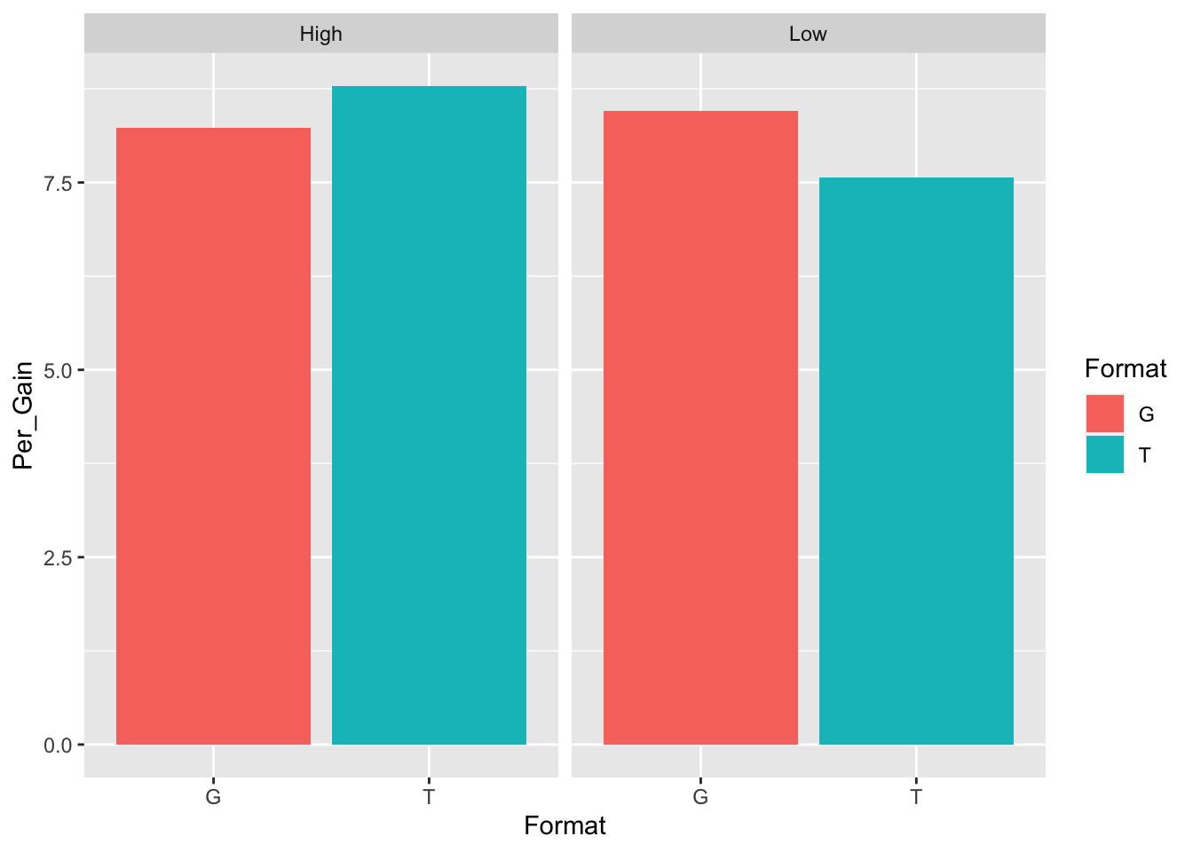
The final thing we want to look at is how high and low learners performed in each of the formats. Here we can see that Low-level learners (<50% correct on the pre-test) performed slightly better in a gloss format than a traditional format. And that high-level learners (>50% correct on the pre-test) performed slightly better in a traditional format. We will need to test if this is statistically signficiant later.
tab3 <- tapply(df$Per_Gain, df[,c("Format","Pre_cat")],mean,na.rm=T)
tab3
## Pre_cat
## Format High Low
## G 0.2166352 0.2223812
## T 0.2253465 0.2045472
7 Simple Parametric Tests
7.1 T-Tests
To look at simple comparison of means between two groups we will use a T-test. IN this example, I will compare means of Per_Gain (Percentage of Vocabulary Gains) between the two groups: traditional and gloss.
t.test(df$Per_Gain~df$Format, paired=FALSE)##
## Welch Two Sample t-test
##
## data: df$Per_Gain by df$Format
## t = 0.23826, df = 143.83, p-value = 0.812
## alternative hypothesis: true difference in means between group G and group T is not equal to 0
## 95 percent confidence interval:
## -0.03128275 0.03985813
## sample estimates:
## mean in group G mean in group T
## 0.2195082 0.2152205It appears that these two groups are the same.
7.2 Effect Size
Coming Soon
7.3 Chi-Square Tests
Coming Soon
7.4 ANOVA
The T-test is nice, but it does not allow us to control for potential differences in course. We can do this with a two-way factorial ANOVA.
#Next we will define our model. Here we are predicting Per_Gain while controlling for Format and Course
fit <- aov(Per_Gain ~  Format + Course + Format:Course, data=df)
summary(fit)
## Df Sum Sq Mean Sq F value Pr(>F)
## Format 1 0.0007 0.00070 0.064 0.800
## Course 1 0.2274 0.22737 20.870 1.03e-05 ***
## Format:Course 1 0.0062 0.00623 0.572 0.451
## Residuals 148 1.6123 0.01089
## ---
## Signif. codes: 0 '***' 0.001 '**' 0.01 '*' 0.05 '.' 0.1 ' ' 1Here we can see that course is a significant predictor of gains. To look at the post-hoc we can use TukeyHSD test below.
# Tukey Honestly Significant Differences
TukeyHSD(fit) # where fit comes from aov()
## Tukey multiple comparisons of means
## 95% family-wise confidence level
##
## Fit: aov(formula = Per_Gain ~ Format + Course + Format:Course, data = df)
##
## $Format
## diff lwr upr p adj
## T-G -0.004287691 -0.03774729 0.02917191 0.8004413
##
## $Course
## diff lwr upr p adj
## 2020-1020 0.0774593 0.04395326 0.1109653 1.03e-05
##
## $`Format:Course`
## diff lwr upr p adj
## T:1020-G:1020 -0.017780438 -0.081706581 0.04614570 0.8878925
## G:2020-G:1020 0.064641189 0.002333693 0.12694869 0.0387902
## T:2020-G:1020 0.072496971 0.010189474 0.13480447 0.0154472
## G:2020-T:1020 0.082421627 0.020114131 0.14472912 0.0042058
## T:2020-T:1020 0.090277409 0.027969912 0.15258491 0.0013574
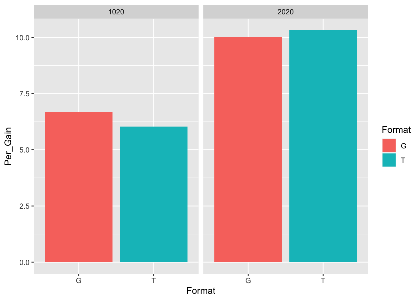
## T:2020-G:2020 0.007855782 -0.052789882 0.06850145 0.9868149These findings show that regardless of format, the 2020 group (second year Chinese course) had a higher percentage of gains than the 1020 gorup.
7.5 Regressions
mod <- lm(Per_Post ~ Per_Pre + Week + Course + VocabWords + Format, df)
summary(mod)
##
## Call:
## lm(formula = Per_Post ~ Per_Pre + Week + Course + VocabWords +
## Format, data = df)
##
## Residuals:
## Min 1Q Median 3Q Max
## -0.26929 -0.06022 -0.01583 0.05494 0.32452
##
## Coefficients:
## Estimate Std. Error t value Pr(>|t|)
## (Intercept) 0.243549 0.093359 2.609 0.0100 *
## Per_Pre 1.029308 0.053570 19.214 < 2e-16 ***
## Week 0.003479 0.004400 0.791 0.4304
## Course2020 0.094231 0.018962 4.970 1.85e-06 ***
## VocabWords -0.002833 0.001673 -1.694 0.0924 .
## FormatT 0.003827 0.017016 0.225 0.8224
## ---
## Signif. codes: 0 '***' 0.001 '**' 0.01 '*' 0.05 '.' 0.1 ' ' 1
##
## Residual standard error: 0.1026 on 146 degrees of freedom
## Multiple R-squared: 0.7576, Adjusted R-squared: 0.7493
## F-statistic: 91.27 on 5 and 146 DF, p-value: < 2.2e-16mod1 <- lm(Per_Post ~ Per_Pre, df)
mod2 <- lm(Per_Post ~ Per_Pre + Course, df)
mod3 <- lm(Per_Post ~ Per_Pre + Course + Format, df)
mod4 <- lm(Per_Post ~ Per_Pre + Course + Format + Format*Per_Pre, df)
anova(mod1,mod2,mod3,mod4)## Analysis of Variance Table
##
## Model 1: Per_Post ~ Per_Pre
## Model 2: Per_Post ~ Per_Pre + Course
## Model 3: Per_Post ~ Per_Pre + Course + Format
## Model 4: Per_Post ~ Per_Pre + Course + Format + Format * Per_Pre
## Res.Df RSS Df Sum of Sq F Pr(>F)
## 1 150 1.8448
## 2 149 1.6123 1 0.232511 21.6239 7.325e-06 ***
## 3 148 1.6119 1 0.000358 0.0333 0.85543
## 4 147 1.5806 1 0.031297 2.9106 0.09011 .
## ---
## Signif. codes: 0 '***' 0.001 '**' 0.01 '*' 0.05 '.' 0.1 ' ' 1summary(mod4)##
## Call:
## lm(formula = Per_Post ~ Per_Pre + Course + Format + Format *
## Per_Pre, data = df)
##
## Residuals:
## Min 1Q Median 3Q Max
## -0.22077 -0.06566 -0.01568 0.05774 0.31830
##
## Coefficients:
## Estimate Std. Error t value Pr(>|t|)
## (Intercept) 0.19197 0.03418 5.617 9.45e-08 ***
## Per_Pre 0.97078 0.06445 15.062 < 2e-16 ***
## Course2020 0.07828 0.01691 4.630 7.97e-06 ***
## FormatT -0.08170 0.04908 -1.665 0.0981 .
## Per_Pre:FormatT 0.17500 0.10258 1.706 0.0901 .
## ---
## Signif. codes: 0 '***' 0.001 '**' 0.01 '*' 0.05 '.' 0.1 ' ' 1
##
## Residual standard error: 0.1037 on 147 degrees of freedom
## Multiple R-squared: 0.7509, Adjusted R-squared: 0.7442
## F-statistic: 110.8 on 4 and 147 DF, p-value: < 2.2e-168 Simple Non-Parametric Tests
8.1 Wilcoxon-Signed Rank Test
Coming Soon
## Loading required package: survival##
## Exact Wilcoxon-Pratt Signed-Rank Test
##
## data: y by x (pos, neg)
## stratified by block
## Z = 10.695, p-value < 2.2e-16
## alternative hypothesis: true mu is not equal to 0## [1] 0.68625## [1] 0.45596159 Basic Graphs
9.1 Bar Graphs
This is a bar chart.
##
## Attaching package: 'ggplot2'
## The following objects are masked from 'package:psych':
##
## %+%, alpha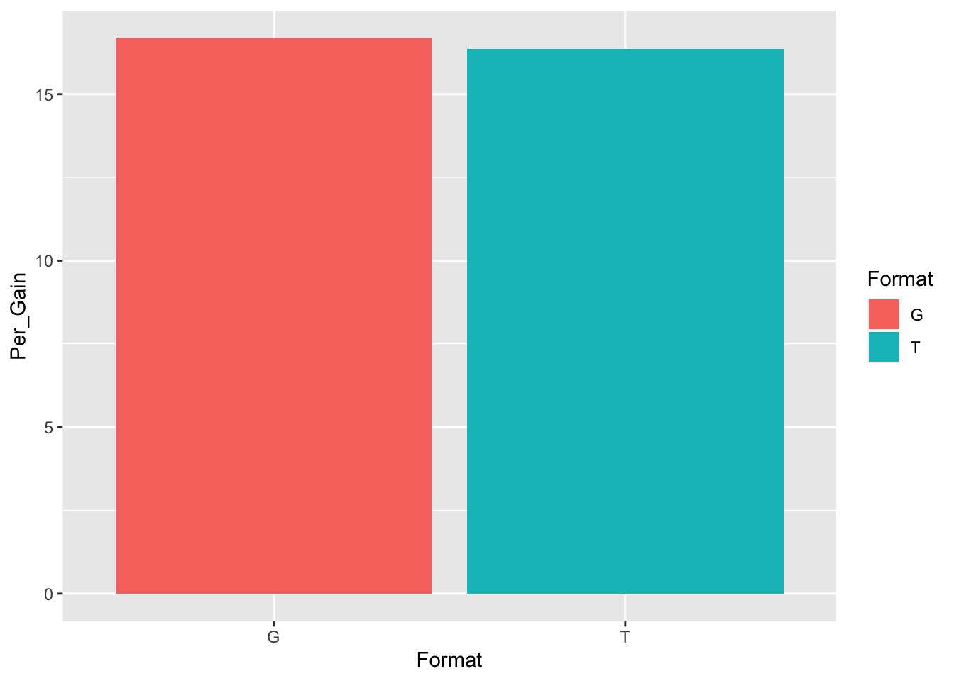
9.2 Box Plots
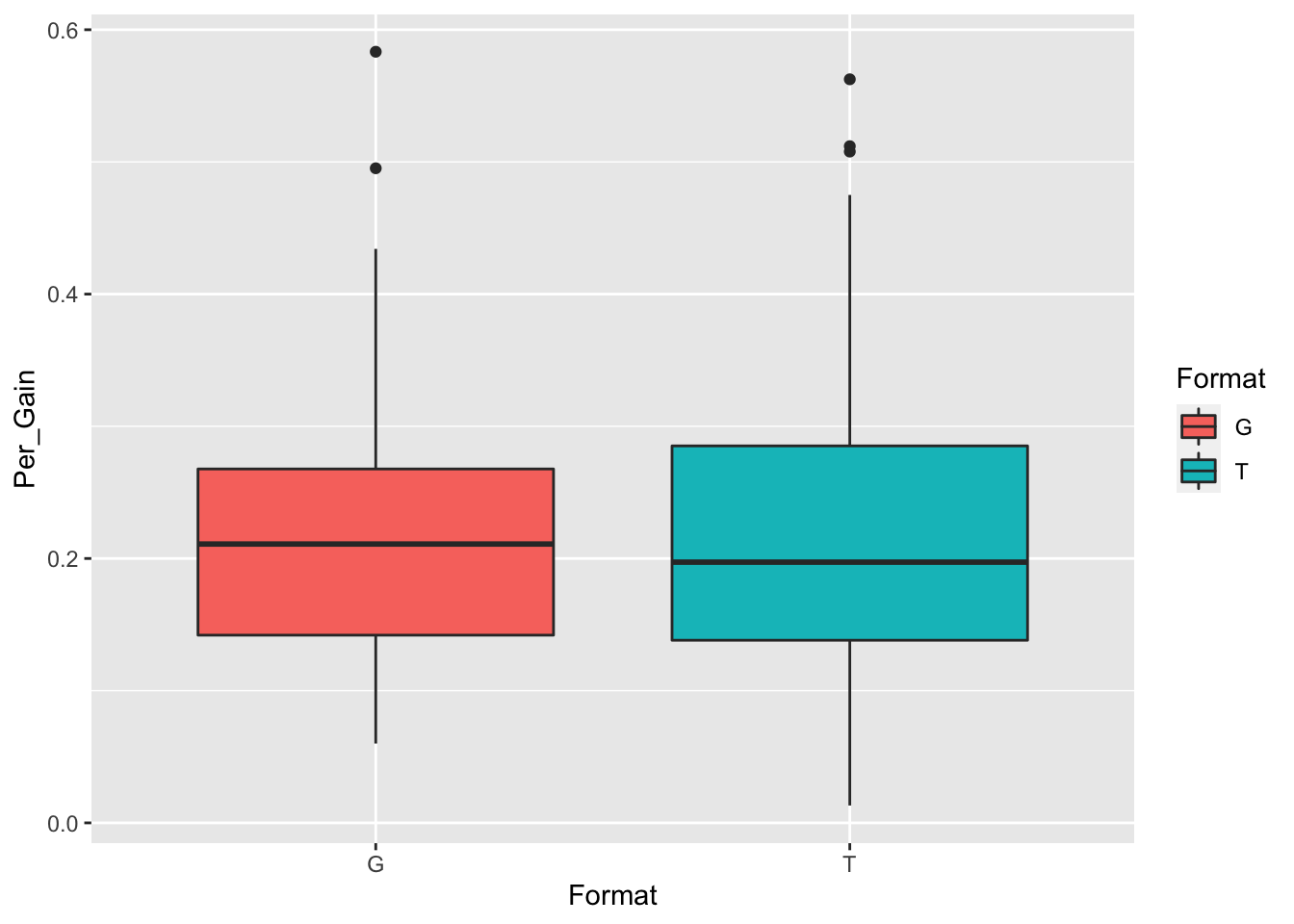
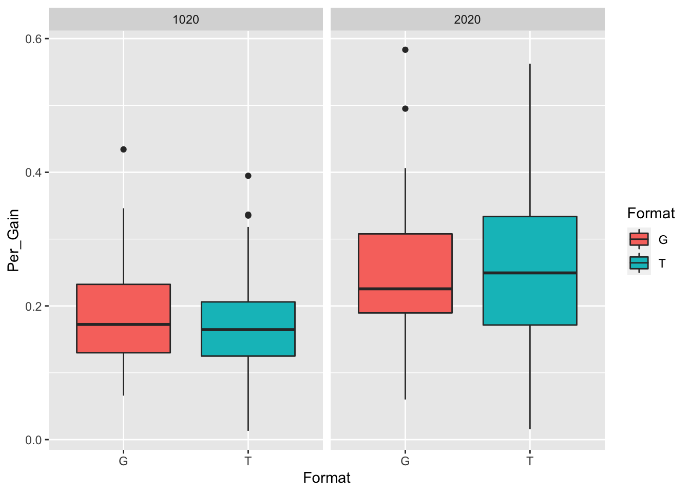
9.3 Linear Plots
f <- ggplot(df, aes(Week,Per_Gain))
f + geom_jitter() + geom_smooth()
## `geom_smooth()` using method = 'loess' and formula = 'y ~ x'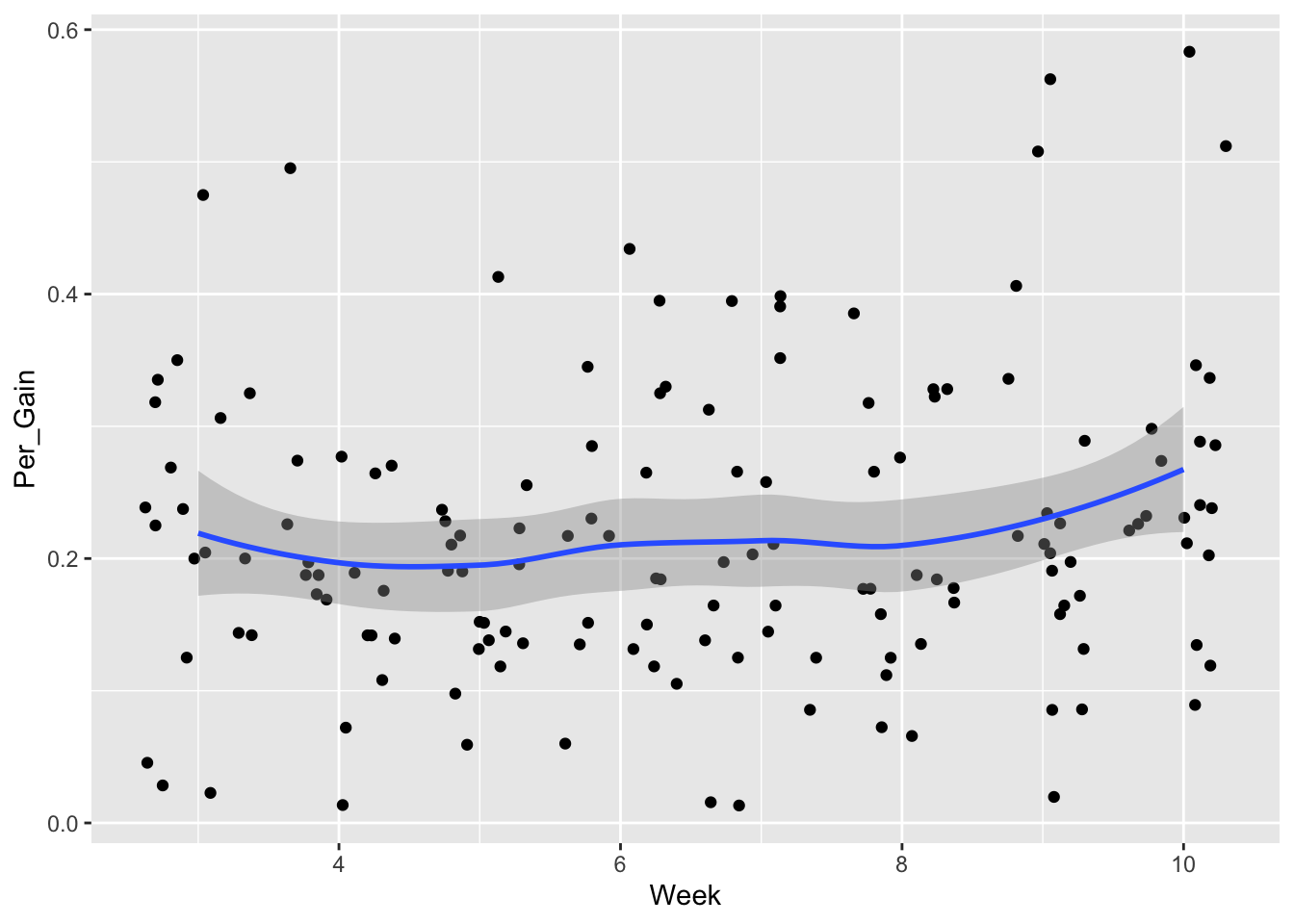
f <- ggplot(df, aes(VocabWords,Per_Gain))
f + geom_jitter(aes(col=Format)) + geom_smooth(method="loess", se=F) +
  labs(title="Vocabulary Gain (%) by Number of New Words", y="Gain (%)", x="Week")
## `geom_smooth()` using formula = 'y ~ x'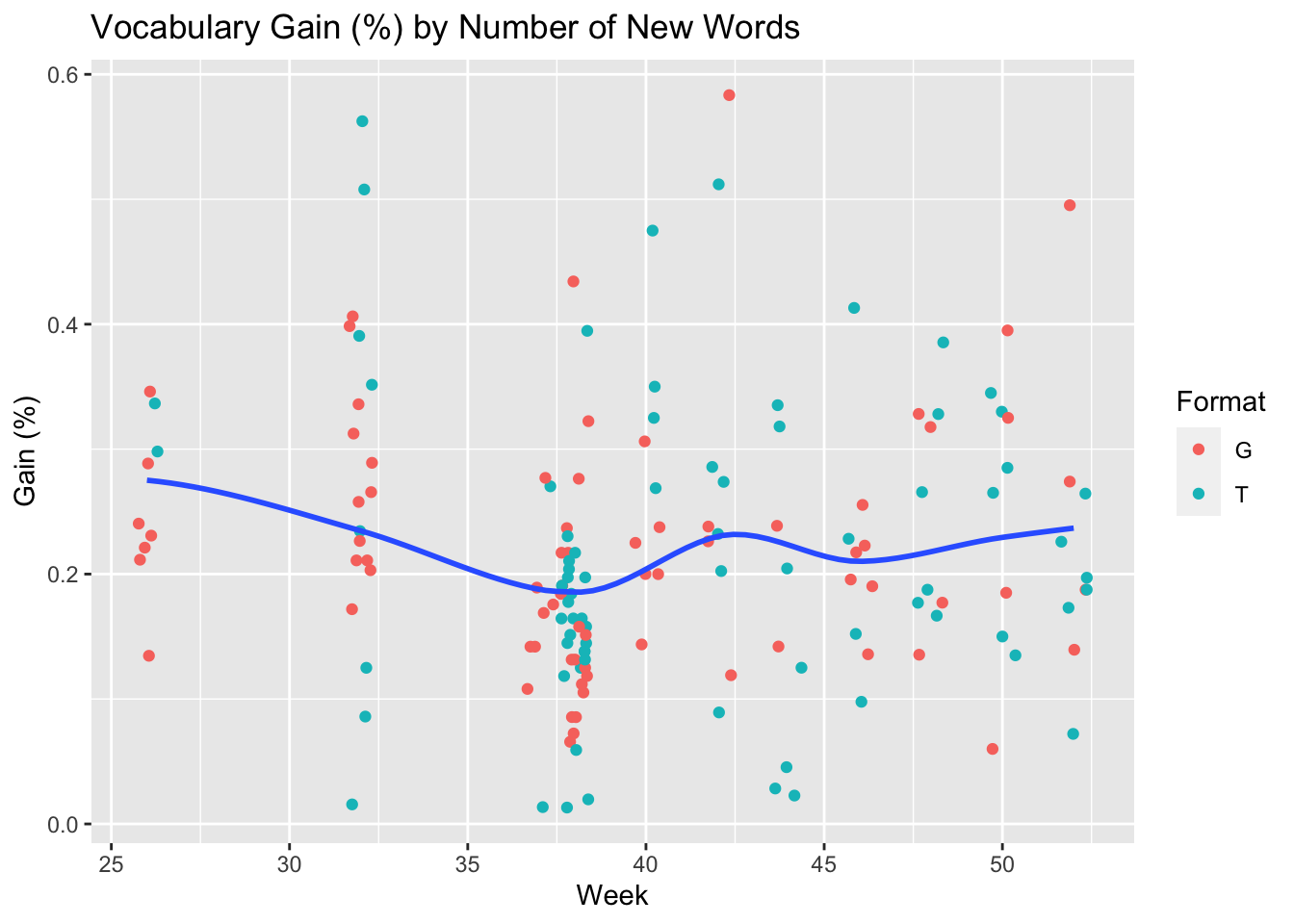
10 Multivariate Analysis
10.1 Path Models
Coming Soon
10.2 Cluster Analysis
Coming Soon
10.3 CART Analysis
Coming Soon
Follow @frdbrick